
Presented here is a very basic social network analysis of four networks completed through Gephi. Gephi is an opensource tool for social network analysis.
Network1
Network Overview
| Density | 0.4 |
| Average degree | 3.6 |
| Diameter | 4 |
Density is 0.4 which means that given the number of nodes there is a possibility of many more connections. However, only 40% of possible connections have materialized.
Network Node Details
| Label | Degree | Closeness Centrality | Betweenness Centrality |
| Bob | 4.00 | 1.89 | 0.83 |
| John | 4.00 | 1.89 | 0.83 |
| Mike | 3.00 | 2.00 | 0.00 |
| Emma | 5.00 | 1.56 | 8.33 |
| Jill | 6.00 | 1.67 | 3.67 |
| Shane | 5.00 | 1.56 | 8.33 |
| Leah | 3.00 | 2.00 | 0.00 |
| Liz | 3.00 | 1.67 | 14.00 |
| Allen | 2.00 | 2.33 | 8.00 |
| Lisa | 1.00 | 3.22 | 0.00 |

Closeness Centrality:
Least value: Lowest values are for Emma and Shane. These nodes as seen in the graph are positioned in such a way in the network that they can reach any other nodes in lesser number of hops as compared to others.
Highest Value: Lisa has the highest value of closeness centrality. As seen in the graph, Lisa is positioned at one end of the network and would need more hops to reach to nodes at the opposite end as compared to others.
Betweeness Centrality:
Highest: Liz has the highest value. As seen in the graph, Liz acts like a network broker between nodes on one end to Lisa and Allen. It is impossible to reach to Allen and Lisa without Liz coming in between.
Lowest: Minimum value is 0 for Mike, Leah and Lisa. As seen in the graph these nodes lie at the periphery of the network and it possible to reach to other nodes bypassing them. In other words they are not needed in between by any of the nodes to access any other node.
Degree:
Jill has highest number of connections with others. As seen in the graph she is connected to six other nodes which is highest for any node. The least is for Lisa as she is at one end of network and has just one connection
Network 2
Network overview:
| Density | 0.208 |
| Average degree | 3.125 |
| Diameter | 5 |
Node Details
| Label | Degree | Closeness Centrality | Betweenness Centrality | Modularity Class |
| Bob | 4.00 | 2.58 | 0.83 | 0.00 |
| John | 4.00 | 2.58 | 0.83 | 0.00 |
| Mike | 3.00 | 2.67 | 0.00 | 0.00 |
| Emma | 5.00 | 2.08 | 15.83 | 0.00 |
| Jill | 6.00 | 2.42 | 3.67 | 0.00 |
| Shane | 5.00 | 2.08 | 15.83 | 0.00 |
| Leah | 3.00 | 2.67 | 0.00 | 0.00 |
| Liz | 3.00 | 1.92 | 35.00 | 0.00 |
| Allen | 3.00 | 2.17 | 32.00 | 1.00 |
| Lisa | 4.00 | 2.67 | 14.00 | 1.00 |
| Tom | 3.00 | 2.75 | 4.50 | 1.00 |
| Merry | 2.00 | 3.50 | 0.00 | 1.00 |
| Mark | 3.00 | 3.42 | 0.50 | 1.00 |
| Jen | 1.00 | 1.00 | 0.00 | 2.00 |
| Sean | 1.00 | 1.00 | 0.00 | 2.00 |
| Mia | 0.00 | 0.00 | 0.00 | 3.00 |

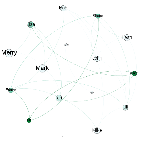
Closeness = denoted by size. Small: Closest; Big: Farthest
Modularity
A total of 4 communities were identified. After Giant component filter two communities remained which are shown here.

Largest community shown in green color comprises of Bob, John, Mike, Emma, Jill, Shane, Leah and Liz. While the second largest consists of Allen, Lisa, Tom, Merry and Mark and it shown in red color.
Jill has maximum number of connections while Mia has no connection. Community that has Jill is evidently the largest community.
In Red community Allen is closest of all while Liz is overall closest to most nodes. Liz also has highest betweeness centrality.
Network 3 from Twitter
| Raw Data | After applying Giant Filter | |
| Nodes | 835 | 593 |
| Edges | 1132 | 1075 |
| Degree | 2.71 | 3.62 |
| Diameter | 8 | 8 |
| Density | 0.003 | 0.006 |
Network Diagrams:


Larger -> high betweenness
Color: Closeness
Darker -> Closer
Modularity
15 communities have been indentified based on resolution of 1. They have been color coded.

Network 4 from Blog
| Raw Data | After applying Giant Filter | |
| Nodes | 194 | 130 |
| Edges | 195 | 191 |
| Degree | 2.01 | 2.938 |
| Diameter | 7 | 7 |
| Density | 0.01 | 0.023 |
Network Diagrams
Edges have been shown in orange color with darkness proportional to weight. Degree ranking are shown in color with dark representing higher degree.

Betweenness Centrality shown in size- larger means highest betweeness while closeness centrality shown in color. Darker means closest.

Modularity
Four communities have been identified as shown in the figure.


Nice tables. Very helpful to compare with the images.